Exploratory Data Analysis With Pandas Profiling

Sharing is caring!

Last Updated on November 19, 2021 by Jay

In this short tutorial, we’ll learn about a data exploratory library – pandas profiling. It’s kinda like the .describe() method in pandas, but much better.

We can use pip install to get the library.

pip install pandas-profiling

Set up coding environment

For this tutorial, we will use Jupyter Notebook, which is also recommended by the pandas_profiling official documentation.

If you don’t want to bother with a virtual environment, go ahead install pandas-profiling system wide on your computer. If you want to follow best practices and use a virtual environment, do the following:

1. Create a virtual environment
2. pip install pandas-profiling ipykernel ipywidgets
3. Link ipykernel with the virtual environment
4. Start coding

Check out this tutorial on how to set up Jupyter Notebook and Virtual Environment. If you don’t want to use the Jupyter Notebook environment, scroll down to the bottom of this tutorial to see how to generate the report as a file.

Data

We are going to use the gapminder dataset which contains years and life expectancy for countries around the world.

import plotly.express as px
from pandas_profiling import ProfileReport

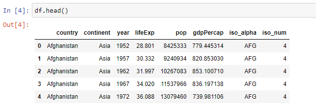
df = px.data.gapminder()

To get a feeling of what’s inside the dataset:

Let’s now put the dataframe into pandas_profiling to generate a report.

profile = ProfileReport(df, title="Pandas Profiling Report", explorative=True)
profile.to_notebook_iframe()

In a few seconds, we should see a Pandas Profiling Report generated in our notebook. There are a few sections in the report: Overview, Variables, Interactions, Correlations, Missing values, Sample.

The Overview section gives a high-level overview of the dataset, including the number of variables (columns), number of observations (rows), the kind of variable types.

The Variables section shows some details about each variable, for example, the number of distinct values, the number of observations for each value, etc.

For each of the variables, we can “Toggle details” to do a deeper dive into a specific data column.

The Interaction section is a quick data visualization. We can switch around the x and y-axis to see how one variable can affect another.

The Correlations section shows a correlation matrix with different coefficient calculations.

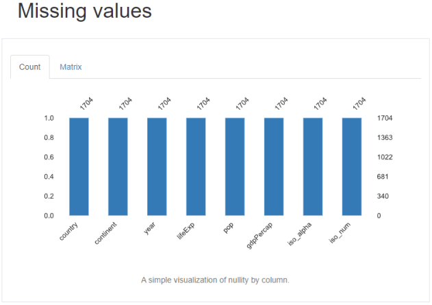
The Missing values section highlights the number of missing (null) values for each data column.

Last but not least, the Sample section shows the top 10 and bottom 10 sample data.

After reviewing this report, we can get a pretty good understanding of the data at hand.

Large Datasets

For large datasets, we can use a minimal=True argument to make to shorten profiling report generation time.

profile = ProfileReport(df, title="Pandas Profiling Report", minimal=True)

Save profiling report as a file

So you don’t want to use the Jupyter Notebook environment, that’s totally fine. We can still use pandas_profiling and generate a report as a webpage HTML file.

profile.to_file(r'C:\Users\jay\Desktop\PythonInOffice\pandas_profiling\output.html')