Last Updated on March 12, 2023 by Jay
This article will walk through a stock price prediction demo using LSTM in Python. how to predict stock prices using LSTM and Python. The basic assumption of any traditional Machine Learning (ML) based model is that all the observations should be independent of each other, meaning there shouldn’t be any association between each data record/row. However, in the case of any time series data, each observation is dependent upon past observations. For example, the stock price in the market depends upon the past day (or days) prices which generally define their trend. However, there are many other factors as well that define the market prices.
We need time series modeling (commonly known as forecasting) to model such time-dependent data. In this article, we will focus on one of the state-of-the-art time series modeling techniques known as Long Short-Term Memory (LSTM). We will cover the basic working of the LSTM and implement it to predict the stock prices in Python. Let’s begin by understanding some details about the algorithm.
What is LSTM and how does it work?
LSTM stands for Long Short-Term Memory, which is an extension of an artificial recurrent neural network (RNN) having the capability to store and learn information over a period of time. Simple right? Of course not. Let’s try to understand from the start. It all started with Neural Networks (NNs), which led to the discovery of RNNs and finally LSTMs.
- Artificial Neural Networks (ANN): You can consider ANN very similar to the brain. Basically, they also consist of neurons that receive information from previous neurons, process them, and then pass it to the next neuron. Based on all the information collected by these neurons, our brain finally makes decisions. ANNs also work the same way as these neurons learn the patterns within data, and improvise enough to predict the next outcome. They form the base of all the deep-learning algorithms and are the main factor why deep learning has become so powerful and popular these days.
- Recurrent Neural Networks (RNN): RNNs are the extension of ANNs with an internal memory unit, meaning it remembers its input and uses it to learn the subsequent inputs more precisely. This makes RNN very apt for any sequential (or time series) datasets.
- Long short-term memory (LSTM): LSTMs are an improvement over RNNs. They operate on a more sophisticated architecture that resolves all the challenges earlier faced by RNNs.


A closer look at LSTM
As shown in the image above, an LSTM layer consists of a set of recurrently connected blocks (commonly known as memory blocks). These blocks are connected to multiple blocks further, and each contains three multiplicative gates known as the input gate, output gate, and forget gate. As the name suggests, these gates work as following
- Input gate controls what new information will be added from the current input
- Output gates decide what to output based on the current memory
- Forget gate decides what information can be thrown away
This architecture makes LSTMs special as they can retain information for a long period of time and also decide when to forget the information. Therefore, we can use LSTM in various applications such as stock price prediction, speech recognition, machine translation, music generation, image captioning, etc.
Stock Price Prediction using LSTM
The best way to learn about any algorithm is to try it. Therefore, let’s experiment with LSTM by using it to predict the prices of a stock. Just to give you some intuition on why LSTM can be useful in predicting stock prices, let’s recall the basic learning of stock markets which is “history tends to repeat itself”. So, if historical patterns are important in predicting the future value of stocks, LSTM is a perfect fit for this use case.
Getting the Data
Getting any stock price is now simple using the Yahoo finance API. Let’s first set up the environment by installing all the required libraries as listed below.
pip install numpy
pip install pandas
pip install sklearn
pip install yfinance
Once installed, let’s import these packages into our environment. For this project I’m using Python 3.9. I don’t recommend using anything older than Python 3.8 as of writing.
# importing libraries
import numpy as np
import pandas as pd
import matplotlib.pyplot as plt
from sklearn.metrics import mean_squared_error
import yfinance as yf
from sklearn.preprocessing import MinMaxScaler
import warnings
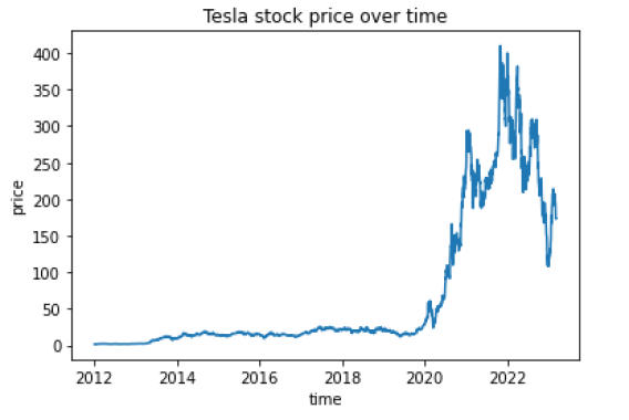
warnings.filterwarnings('ignore')Let’s directly load the stock data for Tesla (TSLA) using the Yahoo finance API. We have filtered the data from the year 2012 to the present, as 10+ years of data is sufficient for our experimentation. As observed, we have the stock price (open, close, high, low) at the daily level and the volume traded.
# download data using Yahoo finance API
df = yf.download('TSLA').reset_index()
df = df[(df['Date'] >= "2012-01-01") & (df['Date'] <= "2023-03-12")].reset_index(drop=True)

Data Preparation for modeling
For the modeling purpose, we will train/predict the stock closing price. We all know that Tesla stock is very volatile, as reflected in the chart below.
# plot closing price over time
plt.plot(df["Date"], df["Close"])
plt.title("Tesla stock price over time")
plt.xlabel("time")
plt.ylabel("price")
plt.show()
For any linear-based model, we need to scale or normalize our data. Therefore, we will use MinMaxScaler, which will transform our data to values ranging from 0 to 1.
# scaling the closing price
# MinMaxScaler => y = (y - min(y))/(min(y) - max(y))
scaler = MinMaxScaler(feature_range=(0,1))
df['scaled_values'] = scaler.fit_transform(df['Close'].values.reshape(-1,1))
Before we put any bet on our models, it is very important to backtest our models using historical data. Therefore, we will divide the data into training and validation (or testing data), which is unseen by the model. For simplicity, let’s keep last year’s data for testing and the remaining data for training.
# split data into train and training set
train_data = df[df['Date'] < '2022-01-01']
test_data = df[df['Date'] >= '2022-01-01']

# plotting the data
plt.figure(figsize=(10,6))
plt.grid(True)
plt.xlabel('Dates')
plt.ylabel('Closing Prices')
plt.plot(df['Date'], df['Close'], 'green', label='Train data')
plt.plot(test_data['Date'], test_data['Close'], 'blue', label='Test data')
plt.legend()

LSTM module expects the data to be in a specific format, usually a 3D array. In this article, we are just going to use the historical price to forecast the next day’s price but you can add other external vectors as well for better model training.
Also, we have selected 60 days lookback period (total days in past to be considered while forecasting price for the next day). Note that you can consider any other look-back period based on your data or experimental observations.
x_train = []
y_train = []

for i in range(60, len(train_data['scaled_values'])):
    x_train.append(train_data['scaled_values'][i-60:i])
    y_train.append(train_data['scaled_values'][i])

x_train, y_train = np.array(x_train), np.array(y_train)

# converting it back to 3D array as required by LSTM
x_train = np.reshape(x_train, (x_train.shape[0], x_train.shape[1], 1))
Here, each x_train is 60 days of stock price and their corresponding y_train variable is the next day’s stock price.
Similarly, let’s transform the test data as well in the required format, which will be used for evaluating model performance.
x_test = []
y_test = test_data['scaled_values']

for i in range(60, len(test_data)):
    x_test.append(test_data['scaled_values'][i-60:i])

x_test = np.array(x_test)
x_test = np.reshape(x_test, (x_test.shape[0], x_test.shape[1], 1))
Introduction to Keras
To set up model training using LSTM, we will use the library Keras. Let’s install and load the required packages.
!pip install kerasfrom keras.models import Sequential
from keras.layers import Dense, LSTM, DropoutWe have imported some modules from Keras. Let’s understand each module in detail.
- Sequential: This is the base function required to initialize any neural network architecture. Post this, we can add multiple layers of networks for the model training.
- Dense: Dense is the fully connected neural network that we are going to use as the final layer to get the final output (prices)
- LSTM: LSTM is the main layer that we are going to tweak and play in our overall architecture
- Dropout: Dropout is a technique where we randomly select neurons that will be ignored during an iteration. This is used to prevent overfitting while training models.
Let’s define our custom architecture with multiple LSTM layers for robust training.
# define model architecture

# Initialize model
model = Sequential()

# LSTM layer 1
model.add(LSTM(units = 50, return_sequences = True, input_shape = (x_train.shape[1], 1)))
model.add(Dropout(0.25))

# LSTM layer 2
model.add(LSTM(units = 50, return_sequences = True))
model.add(Dropout(0.25))

# LSTM layer 3
model.add(LSTM(units = 50, return_sequences = True))
model.add(Dropout(0.25))

# LSTM layer 4
model.add(LSTM(units = 50))
model.add(Dropout(0.25))

# final layer
model.add(Dense(units = 1))
model.summary()

As observed, we have used four LSTM layers in the overall architecture, followed by multiple dropouts to introduce randomness. Each LSTM layer requires the following arguments that need to be defined:
- units are the dimensionality of the output space (we should experiment with multiple units to figure out the best combination for each use case)
- return_sequence is set to true so that the output of the layer will be another sequence of the same length
- input_shape: input shape for the first layer will be the shape of our training data
Here, we have used 0.25 as Dropout, meaning 25% of the layers will be dropped each time to prevent overfitting. This is again a hyperparameter that we will have to tune to identify the best combination.
The Dense layer is the final layer that will return only one output which will be the stock price.
Let’s compile our model.
model.compile(optimizer = 'adam', loss = 'mean_squared_error')In the model.compile, we are using “Adam” optimizer (which is the most common optimizer. However, feel free to try any other optimizer as well. The loss function used here is “mean_squared_error” since we are training a regression model.
Model Training
Once done, let’s finally fit this model on our training data.
model.fit(x_train, y_train, epochs = 10, batch_size = 32)In the model.fit object, we have passed the following arguments:
- x_train: training data (an array containing the historical prices with a lookback of 60 days)
- y_train: next day stock price (which we need to forecast)
- epochs: Total iteration to be conducted. Each iteration means “one pass over the entire dataset”. It is also helpful in logging and evaluating over time
- batch_size: Another hyperparameter that defines the number of samples to work through before updating the internal model parameters
Based on these parameters, the model trains over the defined epochs and prints the overall loss (mean_squared_error). As observed, the model loss has decreased over time. However, it will take some more epochs to converge.
For now, let’s use this model to predict the unseen test data and check how the model performs.
# predict on test data
predicted_stock_price = model.predict(x_test)
predicted_stock_price = scaler.inverse_transform(predicted_stock_price)
Model performance
# plot all the series together
plt.figure(figsize=(10,5), dpi=100)
plt.plot(train_data['Date'], train_data['Close'], label='Training data')
plt.plot(test_data['Date'], test_data['Close'], color = 'blue', label='Actual Stock Price')
plt.plot(test_data[60:]['Date'], predicted_stock_price, color = 'orange',label='Predicted Stock Price')

plt.title('Tesla Stock Price Prediction')
plt.xlabel('Time')
plt.ylabel('Tesla Stock Price')
plt.legend(loc='upper left', fontsize=8)
plt.show()

Woah! As observed, our model can capture the trend pretty well.
Although to compare the actual accuracy/error of the model, we can utilize the below performance matrices to understand the actual model performance.
from sklearn.metrics import mean_absolute_error
import math

y_true = test_data[60:]['Close'].values
y_pred = predicted_stock_price

# report performance
mse = mean_squared_error(y_true, y_pred)
print('MSE: '+str(mse))
mae = mean_absolute_error(y_true, y_pred)
print('MAE: '+str(mae))
rmse = math.sqrt(mean_squared_error(y_true, y_pred))
print('RMSE: '+str(rmse))
mape = np.mean(np.abs(y_pred - y_true)/np.abs(y_true))
print('MAPE: '+str(mape))
The point forecast from our model is giving us 32% MAPE (mean absolute percentage error), which is mediocre. We can definitely improve more on the model as we know only historical prices don’t drive the stock market. Many internal/external factors define the market, which can be captured in the 3D tensor used by LSTMs.
Summary
That was a high-level workflow on using LSTM and Python to predict stock prices. I hope you find it useful. However, you should do your own research and testing before putting any real money based on these algorithms.
Thanks for the useful example.
I have to note that the test is not the most representative, because for each point the historic data are used, so the deviation is never too big compared with historic data. Is it possible to create a test where the input data for the testing would include the data obtained from the prediction of previous period?